
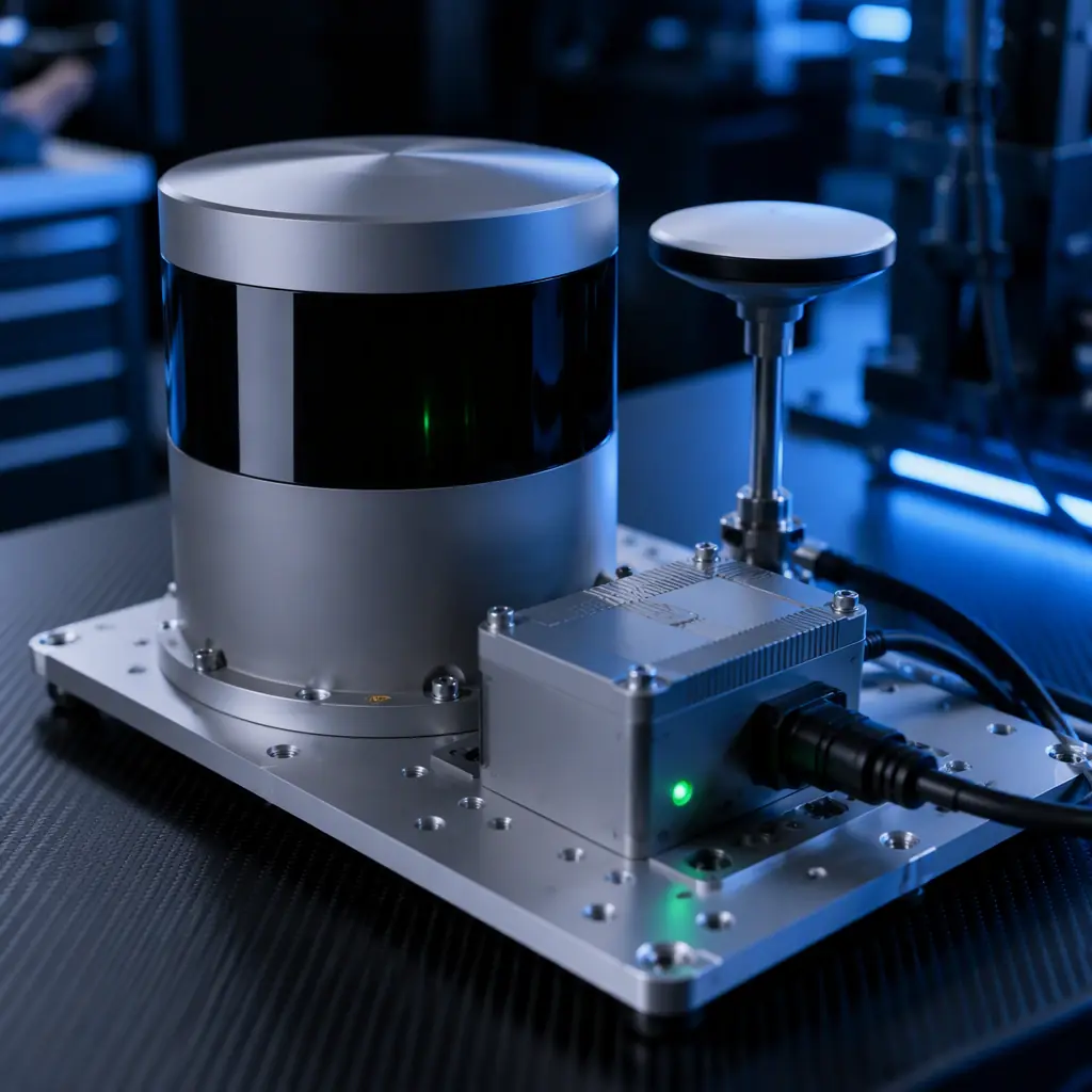
The mapping and survey components guide positions LiDAR as one option among the sensors a survey aircraft carries. This article goes deep on the LiDAR option itself: what the datasheet numbers mean, how the accuracy budget is built, and what to put in the RFQ. If you are deciding between LiDAR and photogrammetry first, start with the mapping guide; this guide assumes the decision has been made and the scanner selection has begun.
Why LiDAR is specified differently from a camera payload
A camera is a passive sensor: it records light that already exists. LiDAR is an active sensor, it emits its own laser pulses and measures the time of flight of each return. That difference drives three procurement consequences:
- The data is georeferenced directly. Every laser return is a range measurement from a known scanner position and attitude, so the point cloud comes out of the processing chain with coordinates already assigned. A photogrammetric model needs tie points and bundle adjustment; a LiDAR point cloud needs trajectory correction and calibration, but no image matching.
- It penetrates vegetation. Laser pulses slip through gaps in foliage and record multiple returns per pulse, which is why LiDAR, not photogrammetry, is the tool for bare-earth mapping under tree canopy. The environmental monitoring guide shows where this capability matters in forestry and vegetation programs.
- It works in low light. LiDAR does not need sunlight, so missions can run in shadow, at dusk or under cloud cover where photogrammetry produces unusable models.
The cost of these advantages is a system, scanner plus IMU plus GNSS plus processing, where every component contributes to the final accuracy, and the weakest component sets the ceiling.
Scanner architecture: mechanical, solid-state and the return question
UAV LiDAR scanners split into two architectural families, and the choice affects reliability, cost and point pattern:
- Mechanical scanners use a rotating mirror or prism to sweep the laser beam. They produce a full circular or elliptical scan pattern, cover a wide field of view (typically 360° in azimuth for survey systems) and generally offer the highest range and pulse rates at a given price point. The rotating parts are the maintenance item, but modern survey-grade units are rated for thousands of operating hours.
- Solid-state scanners steer the beam electronically (MEMS mirrors, optical phased arrays or flash illumination). They have no rotating assembly, which improves robustness and simplifies integration, but their field of view is usually narrower: often 70-90°, which changes the flight planning: more lines and more overlap to cover the same strip width.
The second architecture question is the return capability. Single-return scanners record one reflection per pulse; multi-return scanners record two, three or more (typically up to 3-5). Multiple returns are what make vegetation penetration useful, the first return hits the canopy, intermediate returns hit branches, and the last return reaches the ground. If the mission includes any vegetation, multi-return is not optional.
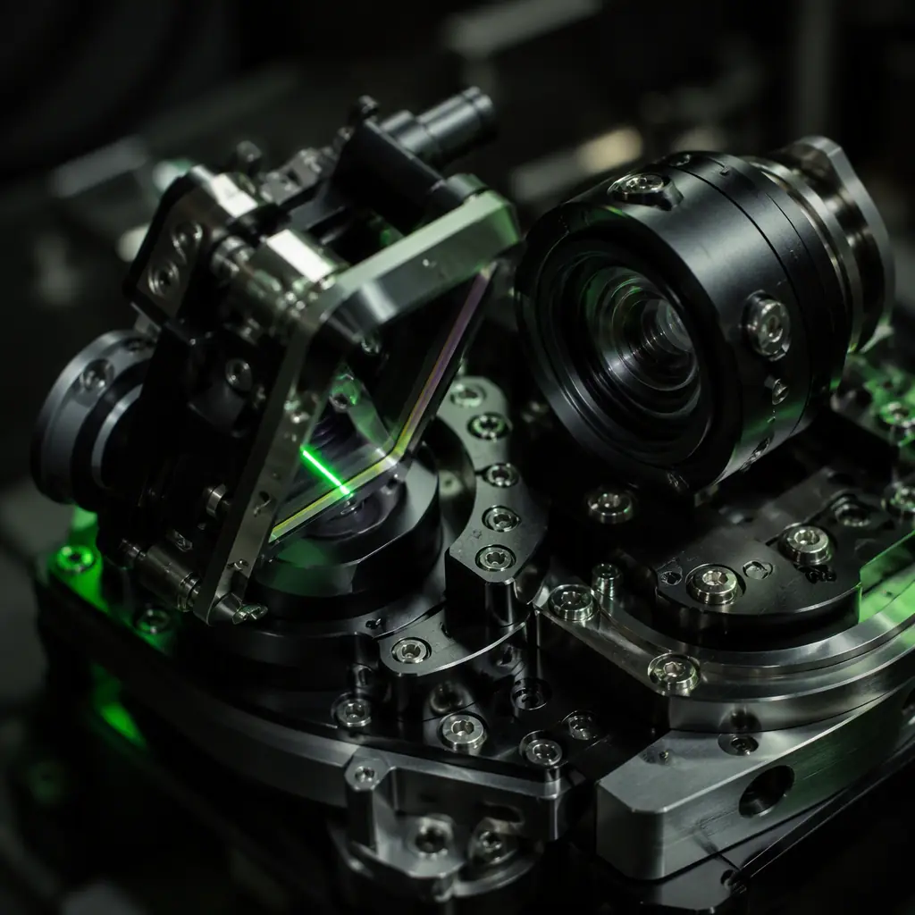 Scanner optical assembly
The accuracy budget: scanner, GNSS, IMU and boresight as one system
The single most misunderstood number in LiDAR procurement is accuracy. The scanner datasheet quotes a ranging precision. But the final point cloud accuracy is a budget that adds several independent error sources:
| Error source | What it is | Typical contribution |
|---|---|---|
| Scanner ranging precision | Per-point distance measurement noise | 0.5-3 cm depending on class |
| GNSS position error | Where the aircraft was when the pulse left | 1-5 cm with RTK/PPK; meters without |
| IMU attitude error | Roll, pitch and heading of the scanner axis | 0.002-0.01° in survey-grade IMUs, grows with range |
| Boresight misalignment | Physical offset and angle between scanner, IMU and GNSS antenna | Eliminated by calibration; 1-3 cm residual if done well |
| Lever arm uncertainty | Distance from GNSS antenna phase center to scanner origin | mm-level when measured; cm-level when guessed |
Notice what this table says: the scanner is only one row. A survey-grade scanner bolted to a non-RTK aircraft produces point clouds accurate to meters, because the GNSS row dominates the budget. The GNSS module selection guide covers the receiver decision; the sensor fusion guide covers how the aircraft estimates its own trajectory, both rows in this budget. When a supplier quotes a payload as "centimeter-accurate," ask which rows are included, under what flight conditions, and with which GNSS correction source.
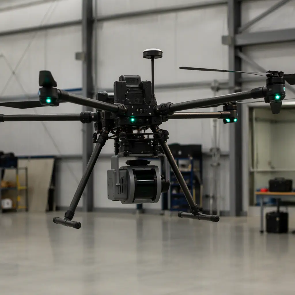 Scanner-IMU-GNSS integration
Point density math: connecting pulse rate to flight speed
Point density (points per square meter) is the number that surveyors actually deliver against, and it is computed from four numbers the procurement team must collect:
- Pulse repetition rate . How many pulses per second the scanner emits (typically 100-1,000+ kHz for modern survey units; more pulses means denser clouds or faster flight).
- Scan rate and field of view . How the pulses are distributed across the swath. A 360° scanner spreads the same pulse rate over more area than a 70° scanner.
- Flight speed . At 10 m/s ground speed, the aircraft advances 10 m every second, stretching the along-track point spacing.
- Flight altitude . Higher altitude widens the swath, spreading the same pulses over more ground.
The practical result: for a given scanner, point density falls as speed and altitude rise. A 600 kHz scanner flown at 50 m and 8 m/s might deliver 300+ points/m²; flown at 100 m and 15 m/s the same scanner might deliver under 100 points/m². The specification conversation is therefore never "which scanner" alone. It is "which scanner, at which altitude and speed, delivering which point density." The flight time estimation guide provides the endurance side of that same flight-planning equation.
Multiple returns and intensity: what they are actually for
Two scanner outputs are routinely oversold or misunderstood at procurement time:
- Multiple returns matter only where pulses penetrate something, canopy, tall grass, wires. In open terrain a multi-return scanner behaves like a single-return one. Specify multi-return for vegetation missions and do not pay for it on bare-earth corridors; conversely, do not accept a single-return scanner for forestry work.
- Intensity records the strength of each return, which correlates with surface reflectivity. Intensity images help classify ground versus vegetation and support line-extraction tasks (paint markings, pavement). Intensity is not calibrated reflectance, it varies with range, angle and scanner settings, so treat it as a classification aid, not a radiometric measurement. For radiometric work the thermal imaging payload guide is the relevant reference.
Fusing LiDAR with imagery: RGB point clouds and camera integration
Most survey LiDAR payloads ship with an integrated camera, and the fusion is a specification issue, not a processing afterthought:
- The camera adds color to the point cloud. Each laser return is projected into the camera frame using the same calibration chain as the boresight. Camera-to-scanner alignment must be calibrated and stable, or the colors smear.
- It also adds the photogrammetric fallback. Many projects deliver both a LiDAR point cloud and an orthophoto from the same flight. The camera and gimbal selection guide covers the imaging side of that dual deliverable.
- Resolution mismatch is the trap. A 60 MP camera produces far more pixels than the LiDAR produces points; the camera captures detail the LiDAR cannot (texture, markings, defects), so the deliverables diverge, the orthophoto shows the road markings, the point cloud shows the bare earth beneath the grass. Specify both deliverables and plan for both.
The processing chain: onboard compute, storage and georeferencing
A LiDAR payload generates data at a rate that surprises first-time buyers: a 600 kHz scanner recording 2-3 returns per pulse plus intensity can produce 5-10 GB per hour of flight, and the processing chain, trajectory smoothing, boresight refinement, point cloud generation, classification, georeferencing, is a desktop workload, not an onboard one. The procurement questions:
- Onboard storage. The payload must hold the full raw data set for the mission; specify storage in hours of flight, not gigabytes, and confirm the write speed keeps up with the pulse rate.
- Onboard processing. Some payloads offer real-time point cloud previews or reduced-density on-the-fly products for field QA. That requires onboard computing capacity, a separate decision from the scanner itself, and one that adds power and weight.
- Post-processing software and workflow. The delivered accuracy depends on the trajectory post-processing (PPK or post-mission correction), so the workflow, software licenses and processing time belong in the RFQ. A payload that needs 10 hours of processing per flight-hour changes the operating cost more than the scanner price does.
- Power and interfaces. A survey LiDAR draws 20-60 W and needs clean, regulated power plus a precise time sync (PPS) connection to the flight controller. The payload power budgeting guide covers the regulator and sequencing decisions; the payload integration guide covers the mechanical and electrical interface standards.
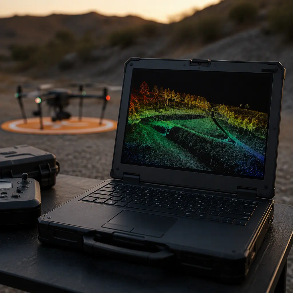 Point cloud processing
Application-driven selection: which scanner for which mission
| Application | Key requirement | Selection consequence |
|---|---|---|
| Corridor mapping (power lines, pipelines, roads) | Range and accuracy at altitude, wire detection | High pulse rate, high range, multi-return for wire extraction |
| Forestry and vegetation | Ground penetration under canopy | Multi-return mandatory, lower altitude flight plan, high point density |
| Terrain and bare-earth survey | Dense, accurate ground points at production speeds | High pulse rate, wide FOV, RTK/PPK GNSS |
| Construction and stockpile volumetrics | Rapid repeat flights, easy processing | Moderate spec sufficient; processing speed and workflow matter most |
| Research and R&D | Configurability, raw data access | Open interfaces, documented formats; see the R&D components guide |
The pattern: missions that fly low and slow (forestry, high-density terrain) can use a smaller, lighter scanner; missions that fly high and fast (corridors, wide-area mapping) need range and pulse rate, which cost weight and power. Payload weight interacts directly with the airframe and endurance decisions covered in the airframe materials guide and the propulsion guides.
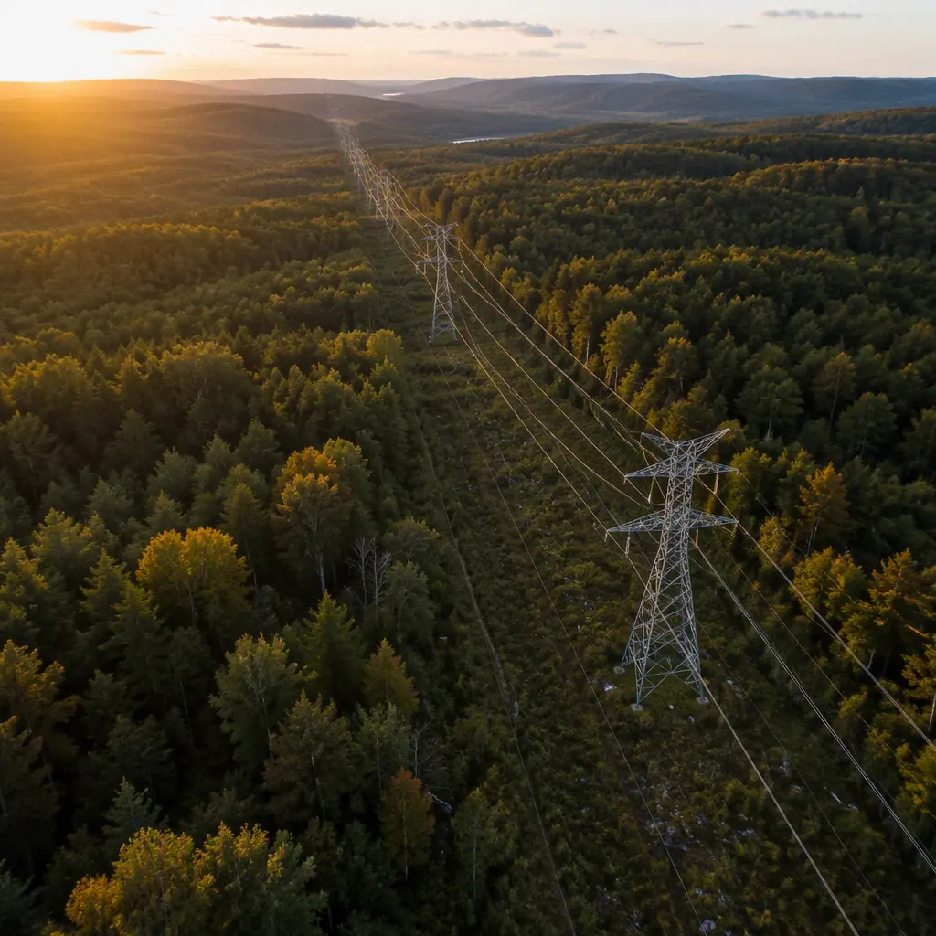 Corridor mapping mission
The LiDAR RFQ checklist
- Scanner specs with conditions. Pulse rate, range, FOV, return count, and the point density the system delivers at the planned altitude and speed, not the headline scanner maximum.
- Accuracy budget in writing. The supplier's stated absolute accuracy with the error-source breakdown: ranging, GNSS (with which correction source), IMU grade, boresight calibration procedure.
- GNSS integration. RTK/PPK compatibility, antenna mounting, lever-arm documentation, and time sync (PPS) interface to the flight controller.
- IMU grade. The IMU specification and its contribution to the error budget at the operating altitude.
- Boresight and calibration. Calibration procedure, tools and the residual error after calibration.
- Camera fusion. Integrated camera resolution, lens, calibration stability and the RGB point cloud output format.
- Storage and processing. Onboard storage hours, processing software, license terms, workflow and processing time per flight-hour.
- Power and interfaces. Draw, voltage range, connector standard, data interface and mounting standard (see the payload integration guide for the interface landscape).
- Environmental rating. Operating temperature range, ingress protection and vibration tolerance for the airframe type.
The bottom line: a UAV LiDAR payload is a system sale, not a sensor sale, the scanner, GNSS, IMU, calibration, processing chain and power integration all sit in the same accuracy budget. Specify the budget as a whole, demand point density at your flight parameters, and put the processing workflow in the RFQ. EMS Drone integrates survey LiDAR payloads end to end, scanner selection, GNSS and IMU matching, power and interface integration, and the calibration and processing workflow, on the airframe your mission needs. Send your survey requirements and target accuracies, and we will respond with the payload specification.
Explore Payloads & Gimbals Back to Blog
The spec trade-offs above come from a real build: on the LiDAR mapping platform we integrated for a survey customer, scanner weight and power draw, not point density, turned out to be the binding constraints on flight time.
Continue Reading
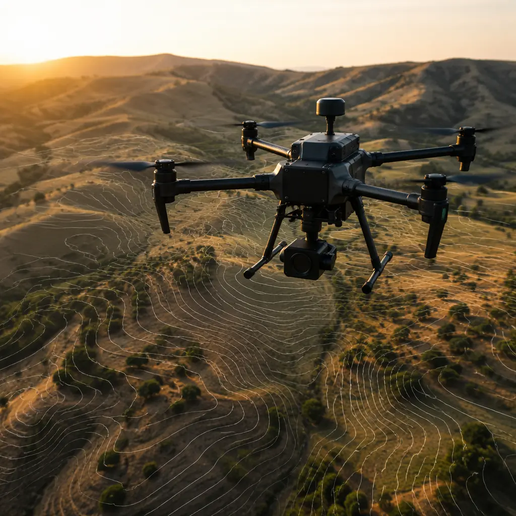
Mapping & Survey Components
Where LiDAR sits in the full survey sensor stack, camera, GNSS and airframe.
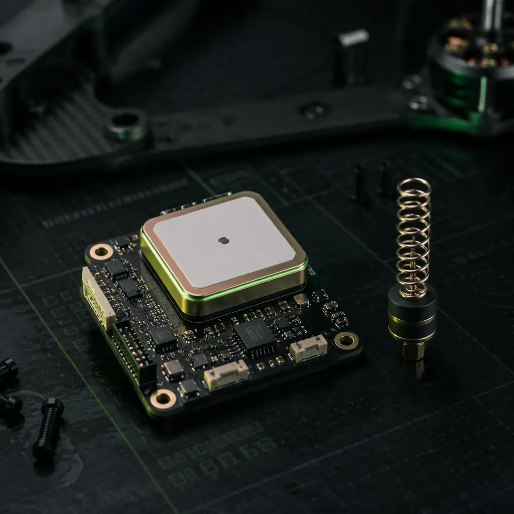
GNSS Module Selection
RTK and PPK receivers, the position row of the LiDAR accuracy budget.
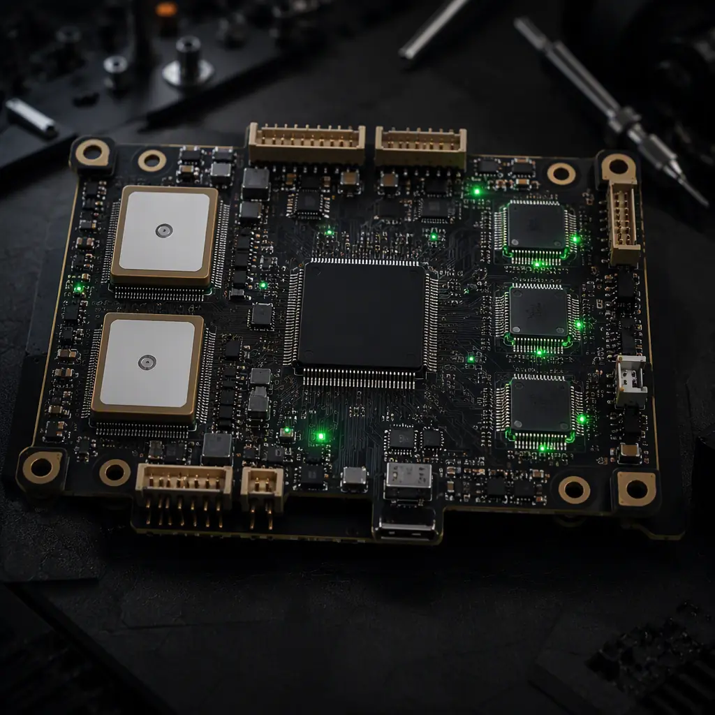
Sensor Fusion & Navigation
How the aircraft's trajectory estimate feeds every LiDAR point.
Edge AI & Onboard Computing
The compute layer for real-time point cloud preview and field QA.
Camera & Gimbal Selection
The imaging half of the RGB point cloud deliverable.